Power spectrum for multiple tracers#
In this tutorial, we will generate a (approximated) halo catalogue with ExSHalos, split the halos into different types of tracers (using their masses), compute all density grids with these tracers, measure all possible power spectra and fit the linear bias using the auto and cross spectra.
After reading this, you will learn:
How to generate a halo catalogue and get the particles displaced with LPT (
pyexshalos.mock.Generate_Halos_Box_from_Pk);How to compute the density grid from a list of tracers with their respective types (
pyexshalos.simulation.Compute_Density_Grid);How to compute all possible power spectra from a list of density grids (
pyexshalos.simulation.Compute_Power_Spectrum);How to compute a theoretical linear halo bias (
pyexshalos.simulation.Get_bh1).
The .py file with the full code is in the github page.
First of all, we need to import numpy, for the manipulation of arrays, pylab, to plot the results, scipy.optimize.minimize, to find the best fit linear biases, and pyexshalos.
# Import the libraries used in this tutorial
import numpy as np
import pylab as pl
from scipy.optimize import minimize
import pyexshalos as exh
Then, we set the parameters of our box and load the linear matter power spectrum from MDPL2 simulation. We also set the parameters of the barrier to the ones found with pyexshalos.utils.Fit_Barrier (described in the generating a halo catalogue tutorial).
# Set parameters for the halo catalogue
Om0 = 0.307115
z = 0.0
nd = 256
Lc = 4.0
L = Lc * nd
Nmin = 1
seed = 12345
verbose = True

# Load the linear matter power spectrum from the MDPL2 simulation
klin, Plin = np.loadtxt("MDPL2_z00_matterpower.dat", unpack=True)

# Best fit parameters found with pyexshalos.utils.Fit_Barrier
params = [0.803958, 0.288991, 0.525464]
Now, we use the parameters above to generate a halo catalogue. Note the inclusion of the OUT_LPT flag. This flag will ask ExSHalos include in the outputed dictionary a field called “pos” with the position of particles displaced with the Lagrangian perturbation theory.
# Generate a halo catalogue with the barrier define above
halos = exh.mock.Generate_Halos_Box_from_Pk(
    k=klin,
    P=Plin,
    nd=nd,
    Lc=Lc,
    Om0=Om0,
    z=z,
    Nmin=Nmin,
    a=params[0],
    beta=params[1],
    alpha=params[2],
    OUT_LPT=True,
    seed=seed,
    verbose=verbose,
)
Attention
Outputting the positions of the particles displaced with LPT will increase the running time and memory! It happens because ExSHalos, by default, compute the displacement only of the particles/cells that belong to a halo with more than Nmin particles.
With the catalogue of halos and particles in hand, we split the halos in different mass bins to simulate the existence of many tracers. The important quantity here is the types array that must have the same size of the total number of tracers and contain intengers that discriminate between the different types of tracers. The mean mass and the number of halos, in each bin, is also computed.
# Define the mass bins to measure the power spectrum
Nh_bins = 7
Mh_bins = np.logspace(
    np.log10(np.min(halos["Mh"])) *
    0.99, np.log10(np.max(halos["Mh"])) * 1.01, Nh_bins
)

# Compute the mean mass and the number of halos in each bin
Mh_mean = np.zeros(Nh_bins - 1)
Nh = np.zeros(Nh_bins - 1)
for i in range(Nh_bins - 1):
    mask = (halos["Mh"] > Mh_bins[i]) * (halos["Mh"] < Mh_bins[i + 1])
    Mh_mean[i] = np.mean(halos["Mh"][mask])
    Nh[i] = np.sum(mask)

# Define the types of halos using the mass bins
types = (np.log10(halos["Mh"]) - np.log10(Mh_bins[0])) // (
    np.log10(Mh_bins[1]) - np.log10(Mh_bins[0])
)
With the type of each halo determined, we compute the density grid of the particles and of each type of halo.
We use the pyexshalos.simualation.Compute_Density_Grid function for it. Relevant options available are:
window: This sets the mass assigment used for the construction of the density grid;interlacing: This sets whether or not to use interlaced grids to alleviate the alising created because of the finite resolution of the grid.
# Measure the density grids
nd = 128
window = "CIC"
interlacing = True

# Particles
grid_p = exh.simulation.Compute_Density_Grid(
    pos=halos["pos"],
    nd=nd,
    L=L,
    window=window,
    interlacing=interlacing,
    verbose=verbose,
)

# Halos
grids_h = exh.simulation.Compute_Density_Grid(
    pos=halos["posh"],
    types=types,
    nd=nd,
    L=L,
    window=window,
    interlacing=interlacing,
    verbose=verbose,
)
Having the density grid of each tracer, we can compute all possible power spectra [N(N+1)/2 for N tracers]. For this we use the function pyexshalos.simulation.Compute_Power_Spectrum. This function can chooses reasonablevalues for the k bins based on the geometry of the grid. However, some options can also be set:
k_min: The left of the k bins used in the measurement;k_max: The right of the k bins used in the measurement;Nk: The number of k bins used in the measurement;ntypes: The number of types of tracers. This quantity does not need to be given in case of only one tracer without interlacing or multiples tracers with interlacing.
# Put the density grid of particles into the same array of halos
grids = np.vstack([grid_p[np.newaxis, :], grids_h])
del grid_p
del grids_h
nh = Nh / L**3

# Measure the Nh_bins*(Nh_bin+1)/2 power spectra
Nk = 32
k_min = 0.0
k_max = 0.3
P_sim = exh.simulation.Compute_Power_Spectrum(
    grid=grids,
    L=L,
    window=window,
    Nk=Nk,
    k_min=k_min,
    k_max=k_max,
    verbose=verbose,
    ntypes=Nh_bins - 1,
)
Now, as a way to visualize the measurements, we fit the linear halo bias, for each mass bin, using the auto power spectrum and the cross spectrum with matter.
# Define some quantities for the computation of chi2
k_NL = 0.1
b0 = 2.0
c0 = 0.0
kdata = P_sim["k"]
Pm = P_sim["Pk"][0]
Pdata = P_sim["Pk"]
Nk = P_sim["Nk"]

# Define the chi2 for fitting the b1
def chi2(theta):
    return np.mean((r - theta[0] - theta[1]*(k/k_NL)**2)**2/err2)/2.0

# Define the gradient of the chi2 above
def chi2_grad(theta):
    pred = theta[0] + theta[1]*(k/k_NL)**2

    return np.array([np.mean((pred - r)/err2), np.mean((pred - r)*(k/k_NL)**2/err2)])

# Fit b1 using Phh and Phm
bhh = []
bhh_err = []
bhm = []
bhm_err = []
count = 1
for i in range(1, Nh_bins):
    # Using Phm
    r = Pdata[count]/Pm
    mask = r > 0.0
    k = kdata[mask]
    r = r[mask]
    err2 = r**2/Nk[mask]
    x = minimize(chi2, jac=chi2_grad, x0=[b0, c0], method="BFGS",
                 options={"maxiter": 1_000})
    bhm.append(x.x[0])
    bhm_err.append(x.hess_inv[0, 0])
    count += i

    # Using Phh
    r = (Pdata[count] - 1.0/nh[i-1])/Pm
    mask = r > 0.0
    k = kdata[mask]
    r = r[mask]
    err2 = (Pdata[count, mask]/Pm[mask])**2/Nk[mask]
    x = minimize(chi2, jac=chi2_grad, x0=[b0**2, c0], method="BFGS",
                 options={"maxiter": 1_000})
    bhh.append(np.sqrt(x.x[0]))
    bhh_err.append(x.hess_inv[0, 0]/(2.0*bhh[-1]))
    count += 1
Warning
The \(\chi {2}\) define above is wrong! It is not taking into account the fact that the halo and particle fields are generated from the same initial conditions. Therefore, the errorbars are expected to be overestimated. We could also consider all power spectra in the estimation of \(b_{1}\) to get smaller errorbars and use the error cancelation properties of multi tracers.
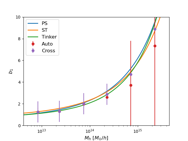
For matter of comparison, we also compute the theoretical linear halo bias, using three standard methods, with the pyexshalos.theory.Get_bh1 function.
# Compute the theoretical linear biases for a few models
Mh_theory = np.logspace(np.log10(Mh_bins[0]), np.log10(Mh_bins[-1]), 600)
b_ps = exh.theory.Get_bh1(M=Mh_theory, model="PS", Om0=Om0, k=klin, P=Plin)
b_tinker = exh.theory.Get_bh1(M=Mh_theory, model="Tinker",
                          theta=300, Om0=Om0, k=klin, P=Plin)
b_st = exh.theory.Get_bh1(M=Mh_theory, model="ST", Om0=Om0, k=klin, P=Plin)
To finish, we plot the measurements and the theoretical models.
# Plot the linear biases
pl.clf()

pl.plot(Mh_theory, b_ps, linestyle="-", linewidth=2, marker="", label="PS")
pl.plot(Mh_theory, b_st, linestyle="-", linewidth=2, marker="", label="ST")
pl.plot(Mh_theory, b_tinker, linestyle="-",
        linewidth=2, marker="", label="Tinker")
pl.errorbar(Mh_mean, bhh, yerr=bhh_err, linestyle="", marker="o",
            markersize=6, label="Auto")
pl.errorbar(Mh_mean, bhm, yerr=bhm_err, linestyle="", marker="o",
            markersize=6, label="Cross")

pl.xlim(Mh_mean[0]*0.5, Mh_mean[-1]*2.0)
pl.ylim(0.0, 10.0)
pl.xscale("log")
pl.yscale("linear")
pl.xlabel(r"$M_{h}$ $[M_{\odot}/h]$", fontsize=12)
pl.ylabel(r"$b_{1}$", fontsize=12)
pl.legend(loc="best", fontsize=12)

pl.savefig("Linear_bias.png")