Generating a halo catalogue#
In this tutorial, we will present, for the first time, how to generate a (approximated) halo catalogue using ExSHalos. We will use the cosmology of the MDPL2 simulation as an example. We will also fit the parameters of the barrier such that the mass function approximates the Tinker’s one.
After reading this, you will learn:
How to compute a theoretical mass function (
pyexshalos.theory.Get_dndlnm);How to fit the ellipsoidal barrier (
pyexshalos.utils.Fit_Barrier);How to generate a halo catologue for a given barrier (
pyexshalos.mock.Generate_Halos_Box_from_Pk);How to measure the mass function of a halo catalogue (
pyexshalos.simulation.Compute_Abundance).
The .py file with the full code is in the github page.
First of all, we need to import numpy, for the manipulation of arrays, pylab, to plot the results, and pyexshalos.
# Import the libraries used in this tutorial
import numpy as np
import pylab as pl
import pyexshalos as exh
Then, we set the parameters that we want for the box and load the linear matter power spectrum. The main parameters here are:
nd: The number of divisions (number of cells) along each direction. You can also pass (nx, ny, nz) to use a different number of cells for each direction;Lc: The size of each cubic cell in Mpc/h;Nmin: The minimum number of particles in each halo. As we will see, Nmin might be any positive integer (even 1!) because all halos in ExSHalos are well resolved;seed: The seed used for the random number generator. This makes the results reproducible.
# Set the parameters for the halo catalogue
Om0 = 0.307115
z = 0.0
nd = 256
Lc = 4.0
L = Lc * nd
Nmin = 1
seed = 12345
x0 = np.array([0.8, 0.3, 0.5])
Max_iter = 100
verbose = True

# Load the linear matter power spectrum of the MDPL2 simulation
k, P = np.loadtxt("MDPL2_z00_matterpower.dat", unpack=True)
To fit the parameters used in the ellipsoidal barrier, we can provide a halo mass function. As an exemple here, we will use the pyexshalos.theory.Get_dndlnm function to compute the Tinker’s mass function. However, note that any mass function can be used, even a non-smooth one from your favorite simulation.
# Compute the theoretical mass function (used as the target mass function here)
Mh = np.logspace(10, 16, 60)
dn_theory = exh.theory.Get_dndlnm(
    M=Mh, model="Tinker", theta=300, Om0=Om0, z=0.0, k=k, P=P
)
Now, we use the utility function pyexshalos.utils.Fit_Barrier to fit the parameters of the barrier to reproduce a given mass function. We can especify some parameters here:
x0: The initial guess for the parameters of the barrier;Max_iter: The maximum number of iterations allowed for the optimization;tol: Tolerance of the error in the fit;
# Fit the parameters of the barrier to reproduce the mass function computed above
params = exh.utils.Fit_Barrier(
    k=k,
    P=P,
    M=Mh,
    dndlnM=dn_theory,
    Lc=Lc,
    seed=seed,
    Nmin=Nmin,
    verbose=verbose,
    x0=x0,
    Max_iter=Max_iter,
)
Attention
Because the effective window used in the halo definition of ExSHalos is not standard (union of top-hat functions in Cartesian coordinates) and the mass discretization is non-uniform (discretazed by the number of cells equidistant to the peak), this function should always be re-run for a new geometry (Lc and nc) of the grid.
With the parameters of the barrier chosen, we proceed to the generation of the halo catalogue through the pyexshalos.mock.Generate_Halos_Box_from_Pk function. (Note that we are using other seed here).
# Generate a halo catalogue with the barrier found above
halos = exh.mock.Generate_Halos_Box_from_Pk(
    k=k,
    P=P,
    nd=nd,
    Lc=Lc,
    Om0=Om0,
    z=z,
    Nmin=Nmin,
    a=params[0],
    beta=params[1],
    alpha=params[2],
    seed=int(seed*23/17),
    verbose=verbose,
)
Note
Note that the halos have any mass value and not just intenger mutipliers of the cell mass!
Just to check that the halo catalogue generated has a halo mass function close to the used, we can measure it using the function pyexshalos.simulation.Compute_Abundance.
# Measure the abundance of the halos
dn_sim = exh.simulation.Compute_Abundance(halos["Mh"], Nm=14, Lc=Lc, nd=nd)
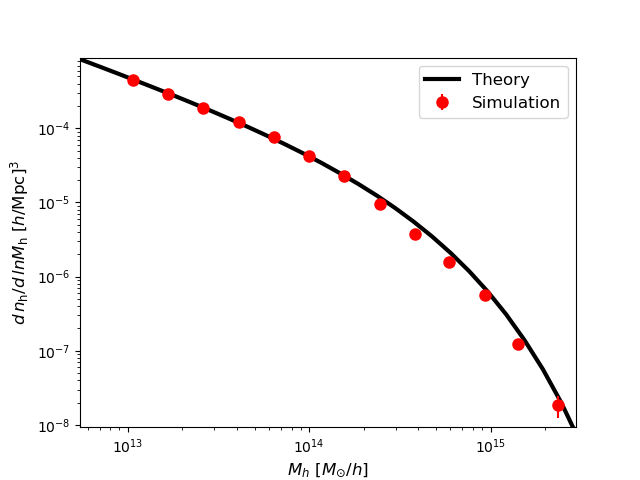
To finish, we plot both the theoretical and simulated mass function to compare them.
# Plot the halo mass function
pl.clf()

pl.plot(
    Mh, dn_theory, linestyle="-", linewidth=3, marker="", color="black", label="Theory"
)
pl.errorbar(
    dn_sim["Mh"],
    dn_sim["dn"],
    yerr=dn_sim["dn_err"],
    linestyle="",
    marker="o",
    markersize=8,
    color="red",
    label="Simulation",
)

pl.xlim(np.min(halos["Mh"]), np.max(halos["Mh"]))
pl.ylim(np.min(dn_sim["dn"][dn_sim["dn"] > 0.0])
        * 0.5, 2.0 * np.max(dn_sim["dn"]))
pl.xscale("log")
pl.yscale("log")
pl.xlabel(r"$M_{h}$ $[M_{\odot}/h]$", fontsize=12)
pl.ylabel(r"$d\, n_{\rm h}/d\, ln M_{\rm h}$ $[h/{\rm Mpc}]^{3}$", fontsize=12)
pl.legend(loc="best", fontsize=12)

pl.show()
Note
Note that the mass function is fine even for the halos with just one particle. This happens because of the semi-analytical nature of ExSHalos. Once we have the barrier, we can give masses to the halos following the mass function of this barrier and the mass interval that the halo belongs. Therefore, to create a halo catalogue with halos resolved (not internally) up to a mass of M, we only need to have a grid with cells/particles with mass M.