HOD for multiple tracers#
In this tutorial, we will generate a catalogue with two types of galaxies tracing the same density field. We are going to use the halo occupation distribution (HOD) with the extension for two tracers presented in appendix C here. We are going to use the best fit parameters that reproduces the red and blue galaxies of IllustrisTNG300.
After reading this, you will learn:
How to generate a halo catalogue (
pyexshalos.mock.Generate_Halos_Box_from_Pk);How to populate the halo catalogue with a HOD (
pyexshalos.mock.Generate_Galaxies_from_Halos);How to split the galaxies into two populations (
pyexshalos.mock.Split_Galaxies);How to compute the density grid from a list of tracers with their respective types (
pyexshalos.simulation.Compute_Density_Grid);How to compute all possible power spectra from a list of density grids (
pyexshalos.simulation.Compute_Power_Spectrum);
The .py file with the full code is in the github page.
First of all, we need to import numpy, for the manipulation of arrays, pylab, to plot the results, and pyexshalos.
# Import the libraries used in this tutorial
import numpy as np
import pylab as pl
import pyexshalos as exh
Then, we set the parameters of our box and load the linear matter power spectrum from MDPL2 simulation. We also set the parameters of the barrier to the ones found with pyexshalos.utils.Fit_Barrier (described in the generating a halo catalogue tutorial).
# Set parameters for the halo catalogue
Om0 = 0.307115
z = 0.0
Nd = 256
Lc = 1.0
L = Lc * Nd
N_MIN = 1
SEED = 12345
VERBOSE = True

# Load the linear matter power spectrum from the MDPL2 simulation
klin, Plin = np.loadtxt("MDPL2_z00_matterpower.dat", unpack=True)

# Best fit parameters found with pyexshalos.utils.Fit_Barrier
PARAMS = [0.803958, 0.288991, 0.525464]
Now, we use the parameters above to generate a halo catalogue.
# Generate a halo catalogue with the barrier define above
halos = exh.mock.Generate_Halos_Box_from_Pk(
    k=klin,
    P=Plin,
    nd=Nd,
    Lc=Lc,
    Om0=Om0,
    z=z,
    Nmin=N_MIN,
    a=PARAMS[0],
    beta=PARAMS[1],
    alpha=PARAMS[2],
    OUT_LPT=False,
    seed=SEED,
    verbose=VERBOSE,
)
Once we have the halo catalogue, we can populate it with galaxies. We use the pyexshalos.mock.Generate_Galaxies_from_Halos function to do so. We use the functional form and parameters from this paper. Note that we set OUT_FLAG=True, this outputs the id of the host halo of each galaxy, using negative ids in the central galaxies.
Note
We also have the extra parameter sigma that sets how the density profile, NFW here, is surpressed for large radii to enforce mass conservation.
# Populate the halos with galaxies
gals = exh.mock.Generate_Galaxies_from_Halos(
    posh=halos["posh"],
    Mh=halos["Mh"],
    nd=Nd,
    Lc=Lc,
    Om0=Om0,
    z=z,
    logMmin=13.25424743,
    siglogM=0.26461332,
    logM0=13.28383025,
    logM1=14.32465146,
    alpha=1.00811277,
    sigma=0.5,
    seed=SEED,
    OUT_VEL=False,
    OUT_FLAG=True,
    verbose=VERBOSE,
)
The galaxies are then split into two populations using the pyexshalos.mock.Split_Galaxies function. We use the parameters of the EFTofLSS analyses with multiple tracerrs that reproduces the halo occupation distribution of blue and red galaxies of the high-resolution IllustrisTNG300 simulation.
# Split the galaxies into two populations
gals_types = exh.mock.Split_Galaxies(
    Mh=halos["Mh"],
    Flag=gals["flag"],
    params_cen = np.array([37.10265321, -5.07596644, 0.17497771]),
    params_sat = np.array([19.84341938, -2.8352781, 0.10443049]),
    seed = SEED,
    verbose = VERBOSE,
)
The density grids and spectra of the tracers are computed using the pyexshalos.simulation.Compute_Density_Grid and pyexshalos.simulation.Compute_Power_Spectrum functions. As in the previous tutorials.
# Compute the density grids
WINDOW = "CIC"
INTERLACING = True
grids = exh.simulation.Compute_Density_Grid(
    pos=gals["posg"],
    types=np.abs(gals_types),
    nd=Nd,
    L=L,
    window=WINDOW,
    interlacing=INTERLACING,
    verbose=VERBOSE,
)

# Measure the power spectra
NK = 32
K_MIN = 0.0
K_MAX = 0.3
P_sim = exh.simulation.Compute_Power_Spectrum(
    grid=grids,
    L=L,
    window=WINDOW,
    Nk=NK,
    k_min=K_MIN,
    k_max=K_MAX,
    verbose=VERBOSE,
    ntypes=2,
)
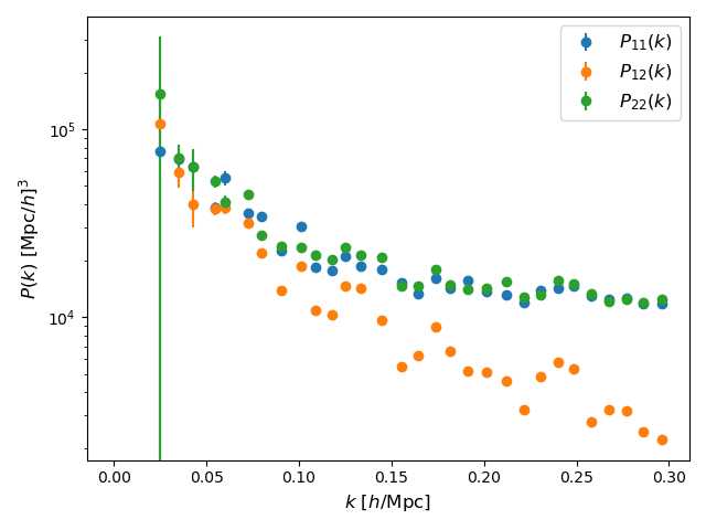
Finally, we plot the power spectra.
# Plot the power spectra
pl.clf()

pl.errorbar(P_sim["k"],
            P_sim["Pk"][0],
            yerr=P_sim["Pk"][0]/P_sim["Nk"],
            linestyle="",
            marker="o",
            markersize=6,
            label=r"$P_{11}(k)$",
            )
pl.errorbar(P_sim["k"],
            P_sim["Pk"][1],
            yerr=P_sim["Pk"][1]/P_sim["Nk"],
            linestyle="",
            marker="o",
            markersize=6,
            label=r"$P_{12}(k)$",
            )
pl.errorbar(P_sim["k"],
            P_sim["Pk"][2],
            yerr=P_sim["Pk"][2]/P_sim["Nk"],
            linestyle="",
            marker="o",
            markersize=6,
            label=r"$P_{22}(k)$",
            )

pl.xscale("linear")
pl.yscale("log")
pl.xlabel(r"$k$ [$h/$Mpc]", fontsize=12)
pl.ylabel(r"$P(k)$ [Mpc$/h]^{3}$", fontsize=12)
pl.legend(loc="best", fontsize=12)

pl.tight_layout()
pl.savefig("Multi_hod.png")
Attention
Note that the power spectra both tracers are very similar. It happens because our simulation has a very low mass resolution, in comarions to the IllustrisTNG300 simulation. For a fair comparison, we should use the same resolution of the original simulation.